
1. Introduction
The “Demystifying Machine Learning Challenges” is a series of blogs where I highlight the challenges and issues faced during the training of a Machine Learning algorithm due to the presence of factors of Imbalanced Data, Outliers, and Multicollinearity.
In this blog part, I will cover Imbalanced Datasets. For other parts, refer to the following links:
– Demystifying Machine Learning Challenges: Outliers
2. What is Imbalanced Data?
Imbalanced data in machine learning refers to the situation where the distribution of classes in the target variable is not equal. This can occur in both binary and multiclass classification problems:
- in a binary classification problem, one class may have significantly more instances than the other class.
- in a multiclass classification problem, one or more classes may have significantly fewer instances than the other classes.
If not addressed correctly, it can lead to biased decision boundaries, inaccurate predictions, and misleading model performance.
What causes Imbalanced Data?
There are mainly two reasons that lead to an imbalanced dataset:
– it is the nature of the problem itself.
– there are biases in data collection or sampling methods.
Below are some real-world problems that involve imbalance data:
- The Fraudulent Transaction Detection problem is a typical example of imbalanced data, as most transactions are genuine while only a small fraction is fraudulent.
- In an Ad Serving and Click Prediction problem, since most users do not click on ads, the majority of data belongs to non-clickers and only a small portion belongs to clickers.
3. Effect on Decision Boundary & Predictions
Imbalanced data can cause classification algorithms to have a biased decision boundary. As such the algorithms may favor the majority class, leading to poor performance and low prediction accuracy for the minority class.
We will look at the effects on common ML algorithms one by one:
(Note: I will mostly skip the mathematics behind the algorithms)
a) Logistic Regression
Logistic Regression tries to find a decision boundary that best separates the two classes of data. The optimization process involves maximizing the log odds or minimizing the log losses. Both the groups try to PUSH the decision boundary, as much as possible, from them. When one class has many more samples than the other, the PUSH force will be dominated by the majority class, and the decision boundary is shifted towards the minority class. This shift towards the minority class may introduce some bias in the prediction of the minority class when the default threshold of 0.5 is used. Unless the class imbalance is extreme, some adjustments in the decision threshold can mitigate the bias.
Verdict: Unless the class imbalance is extreme, Logistic Regression works well with little adjustments in the decision threshold.
b) KNN
KNN classifies a sample based on the majority class among its K nearest neighbors. When K is small, it considers a small number of neighbors to make the classification decision, and when K is large, it considers a large number of neighbors to make the decision. As such, the sensitivity of KNN for imbalanced data also depends on the value of K.
When K is small, KNN is less sensitive to imbalanced data because it considers only a small number of neighbors for classification. When K is large, KNN is more sensitive to imbalanced data because it is more likely that a sample’s nearest neighbors will belong to the majority class, even if the sample itself belongs to the minority class.
Verdict: The level of impact depends on the value of K.
c) Naive Bayes
Naive Bayes computes the probability of sample x belonging to class C as follows:
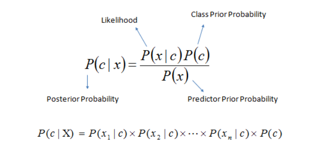
The posterior probability depends on the value of the prior probability. For imbalanced data, the posterior probability of the majority class will be higher than the minority class. As such, no matter what the value of likelihood is, the chances of the posterior probability of the majority class ending up greater than the posterior probability of the minority class is high, leading to biased predictions of the minority class.
Verdict: Naive Bayes is affected by imbalanced data.
d) Decision Tree
Decision Trees recursively splits the data based on feature values that best separate the classes into groups with minimum impurity. Although imbalanced data can affect the split points chosen by the algorithm, all the classes are taken into account at each stage of splitting. As such, imbalanced data do not have any major impact on the algorithm and perform pretty well.
Verdict: Decision Tree algorithm is not heavily impacted by imbalanced data.
4. Misleading Performance Metrics
When it comes to imbalanced data, some metrics can give very misleading results. Hence it is important to understand the limitations of a metric before using it.
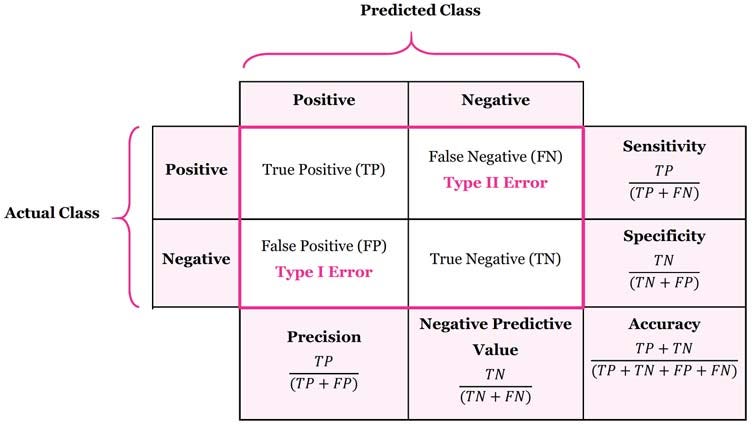
a. Accuracy:
It is defined as the ratio of the number of correct predictions to the total number of predictions. It is calculated as:
Accuracy = (True Positive + True Negative) /
           (True Positive + True Negative + False Positive + False Negative)
Let’s say we have a dataset with 90% negative class samples and 10% positive class samples. A model that always predicts the negative class will have a high accuracy of 90%, even though it is not actually performing well and objectively only predicts one class. As such, Accuracy should not be used with imbalanced datasets.
b. Precision
It is defined as the ratio of the number of true positive predictions to the total number of positive predictions. It gives the answer to “What proportion of positive identifications is actually correct?”. Mathematically, Precision is defined as:
Precision = True Positives / (True Positives + False Positives)
Precision is a useful metric in cases where the cost of False Positives is high. In the Spam Email Detection problem, it is critical to minimize the number of False Positives, i.e., legitimate emails mistakenly identified as Spam. High Precision ensures that Spam emails are identified accurately, reducing the risk of missing out on important messages.
c. Recall or Sensitivity
It is defined as the ratio of the number of true positive predictions to the total number of positive samples. It gives the answer to “What proportion of actual positives was identified correctly?”. Mathematically, Recall is defined as:
Recall = True Positives / (True Positives + False Negatives)
Recall is a useful metric in cases where the cost of False Negatives is high. In the Ad Serving & Click Prediction problem, it is critical to minimize the instances when a user is interested in an ad, but the model fails to predict it as such, and the ad is not served to the user. In such a scenario, the advertiser loses a potential customer, and the ad platform loses potential revenue. High Recall ensures that the platform is serving relevant ads to users who are interested in them.
Note: It is important to note that Precision and Recall are often in tension, meaning that improving one metric often comes at the cost of the other. Therefore, the choice between Precision and Recall as the primary metric depends on the problem at hand and the costs associated with False Positives and False Negatives.
d. F1-Score
It is defined as the harmonic mean of precision and recall. It provides a balanced measure of a model’s ability to identify positive samples while minimizing the number of both False Positives and False Negatives.
F1 Score is calculated as:
F1 Score = 2 * (Precision * Recall) / (Precision + Recall)
In practical terms, a high F1 score indicates that the model is performing well at both identifying positive samples (High Recall) and correctly labeling them as positive (High Precision).
e. AUC
AUC stands for “Area under the ROC Curve”. It provides an aggregate measure of the model’s performance across all possible classification thresholds by calculating the area under the ROC curve. Another way to interpret it is as the probability that the model correctly ranks a positive sample higher than a negative one across all possible classification thresholds.
Let’s say we have a dataset with 90% negative class samples and 10% positive class samples. A model that always predicts the negative class would achieve a very high True Negative Rate, and a very low False Positive Rate. This leads to a curve that is closer to the top left corner of the ROC plot, resulting in a high AUC score. But the model would completely fail to identify any positive samples, resulting in a low Recall and F1 Score. As such, AUC can give misleading scores when dealing with imbalanced data.
Verdict:
- Accuracy and AUC are not well suited for imbalanced data.
- Precision, Recall, and F1 Score provide a more balanced evaluation.
5. Techniques to Handle Imbalanced Data
The are several techniques that can be implemented to reduce the effect of imbalanced data. They can be broadly divided into two groups: data-level techniques and algorithm-level techniques.
Note: As there are already a plethora of blogs explaining these techniques, I will only give a brief rundown.
a. Data-Level Techniques:
Data-level techniques involve modifying the dataset to create a more balanced distribution of classes. The 3 most popular methods are:
- 1. Oversampling: It involves randomly selecting examples from the minority class, with replacement, and adding them to the dataset to increase their representation in the dataset.
- 2. Under sampling: It involves randomly removing samples from the majority class to reduce their representation in the dataset.
- 3. SMOTE: The synthetic minority oversampling technique involves generating synthetic samples to augment the minority class.
Resampling techniques can however result in overfitting and underfitting issues, and care must be taken to ensure that the resulting dataset is representative of the underlying population.
b. Algorithm-Level Techniques:
This method involves tweaking the ML algorithms to tackle imbalanced data.
- Cost-sensitive learning: It focuses on assigning different costs to misclassification errors for different classes. For example, in a Cancer Detection problem, failing to detect cancer (False Negative) may have a higher cost than incorrectly predicting that a person has cancer (False Positive). By assigning different costs to the errors, the model can be optimized to reduce the overall cost of misclassification.
- Using class weights to automatically adjust the weights according to class frequencies is another way to handle the issue.
In addition to the above two techniques, careful consideration of appropriate evaluation metrics also plays an important role in obtaining accurate and reliable predictions.
6. Conclusion
In this blog post, we tried to understand the causes and consequences of imbalanced data on various machine learning algorithms, as well as explored different techniques to address the issue.
Thanks for reading the blog. Please leave comments, feedback, and suggestions, if you feel any. You can reach out to me through my Portfolio or find me on LinkedIn.